Normal Distributions and Z-Scores

The bell curve and the empirical rule

A normal distribution is symmetric and bell-shaped, centered at its mean. The empirical rule describes how the data spreads out around that mean: about 68% of values fall within 1 standard deviation, about 95% within 2 standard deviations, and about 99.7% within 3 standard deviations.

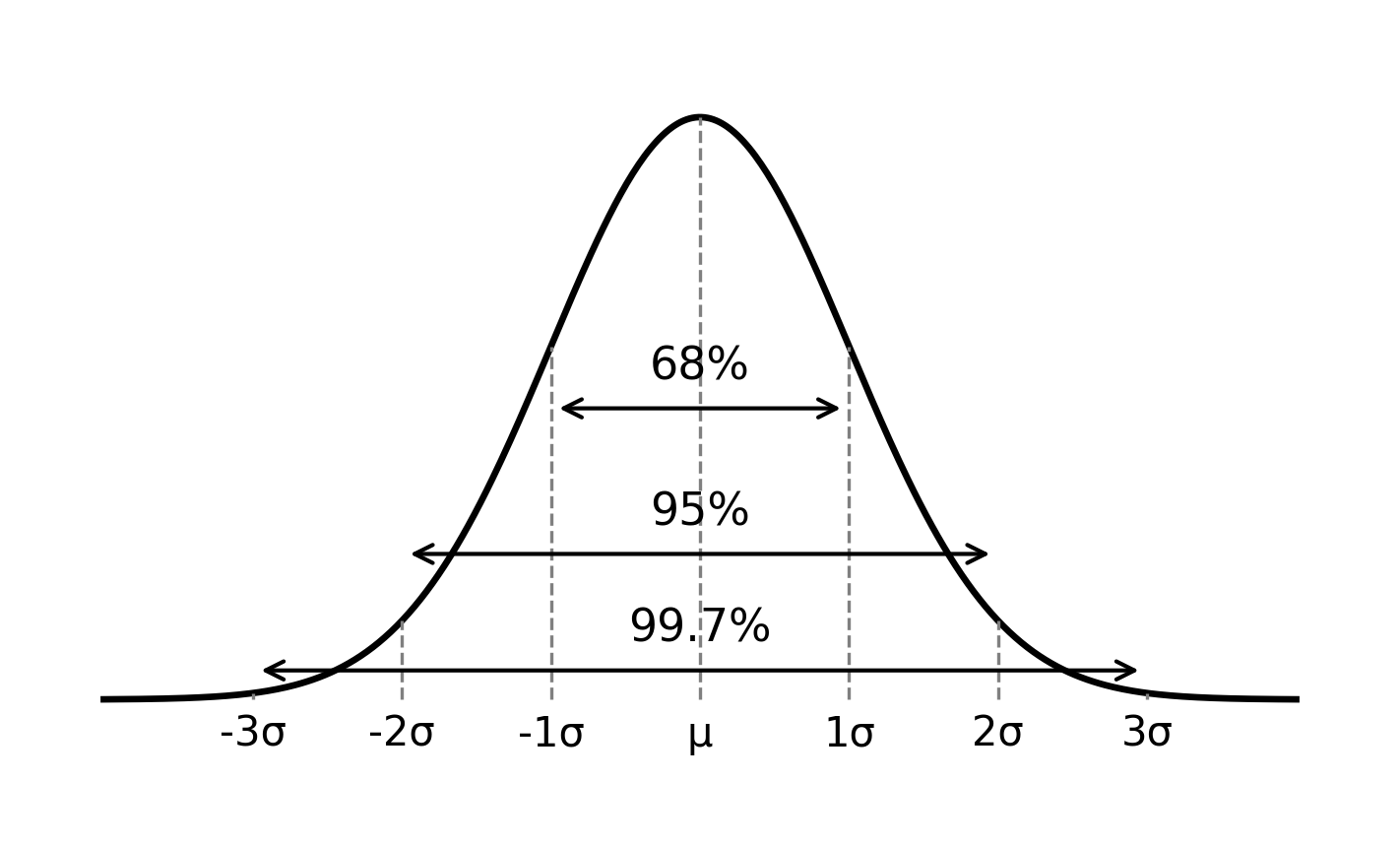
Because the curve is symmetric, each half of a region holds half of its percentage. About 34% of values lie between the mean and 1 standard deviation above it, about 47.5% between the mean and 2 standard deviations above it, and exactly 50% lie above the mean.

The 68-95-99.7 rule is a normal-distribution approximation, not a universal rule for every data set. Use it only when the distribution is stated or reasonably described as normal, or approximately normal. Knowing only a mean and a standard deviation is not enough to assume the empirical rule applies; a strongly skewed distribution with the same mean and standard deviation would not follow the same pattern.

Z-scores

A z-score measures how many standard deviations a value sits from the mean:

$z = \frac{x - \mu}{\sigma}$

Here $x$ is the data value, $\mu$ is the mean, and $\sigma$ is the standard deviation. A positive z-score means the value is above the mean; a negative z-score means it is below. Reversing the formula recovers the original value from a known z-score: $x = \mu + z\sigma$. Keep the sign on $z$ when you use this form, so a z-score of $-2$ means subtracting two standard deviations.

Worked example. A distribution has mean 72 and standard deviation 9. Find the z-score for a value of 90.

$z = \frac{90 - 72}{9} = 2$. The value 90 is 2 standard deviations above the mean.

Applying the empirical rule

The rule is a three-step routine: find how many standard deviations each boundary is from the mean, match that number to 68, 95, or 99.7, and adjust for tails if the question asks about "above" or "below."

Worked example. A distribution is normal with mean 500 and standard deviation 80. Approximately what percent of values fall between 420 and 580?

420 is 1 standard deviation below the mean and 580 is 1 standard deviation above it, so about 68% of values fall in this interval.

Recognize, set up, solve, check. Take a distribution with mean 82 and standard deviation 6, and ask for the percent of values between 70 and 94. Both boundaries are the same distance from the mean, so compute that distance in standard deviations: 70 is $\frac{82-70}{6} = 2$ standard deviations below and 94 is $\frac{94-82}{6} = 2$ standard deviations above. That matches the 95% rule, not the 68% rule (1 SD) or the 99.7% rule (3 SD). No calculator is needed. The common error is assuming the 68% rule applies because the interval looks narrow, without actually computing how many standard deviations away each boundary sits.

Tails

Questions about "above" or "below" a single boundary use the leftover percentage. If 68% of values are within 1 standard deviation, then 32% lie outside, split evenly between two tails: 16% in each. So in a normal distribution, about 16% of values are more than 1 standard deviation above the mean, and about 84% are below that point. For 2 standard deviations, 5% lie outside and 2.5% are in each tail. Always ask which side of the boundary the question wants, because the tail and its complement differ enormously.

Worked example. Heights in a population are approximately normal with mean 66 inches and standard deviation 3 inches. About what percent of people are taller than 72 inches?

$z = \frac{72 - 66}{3} = 2$, so 72 is 2 standard deviations above the mean. About 95% of values lie within 2 standard deviations, so 5% lie outside and half of that, about 2.5%, are taller than 72 inches. A quick sanity check: 72 is far out on the right side of the bell, so a small percentage is what we expect.

It also helps to turn the rule around. If a question tells you that about 16% of values lie above some boundary, that boundary must be 1 standard deviation above the mean, and the distance from the mean to the boundary is the standard deviation. Likewise, if the boundary has a known z-score, you can solve $x = \mu + z\sigma$ for whichever of $x$, $\mu$, or $\sigma$ is missing.

Comparing values from different distributions

Z-scores put values from different distributions on the same scale. A student who scores higher relative to their own test's mean and spread has the higher z-score, even if the raw score is numerically lower. A score of 82 on a test with mean 75 and standard deviation 5 has a z-score of 1.4. A score of 88 on a test with mean 80 and standard deviation 6 has a z-score of about 1.33. The first score is relatively higher, even though it is lower numerically.

Traps to avoid

• Reporting the raw difference $x - \mu$ without dividing by the standard deviation.
• Dropping the negative sign on a z-score for a value below the mean.
• Adding instead of subtracting when the z-score is negative in $x = \mu + z\sigma$.
• Applying the 68% rule when the boundaries are really 2 standard deviations away.
• Giving the percent in the wrong tail, or forgetting to split the outside percentage between the two tails.
• Comparing raw scores from different tests instead of comparing z-scores.