Exponential Models and Exponent Rules

Linear change adds the same amount each step. Exponential change multiplies by the same factor, and that one difference is why it eventually outruns anything that merely adds.

The last shape in this domain is the steepest. A linear relationship grows by adding a fixed amount at each step; an exponential one grows by multiplying by a fixed factor. That single change, addition to multiplication, produces a curve that starts slowly and then climbs without limit, and it models the things in the world that compound: populations, money at interest, the spread of something through a network. To handle it you need the rules for exponents, the form of an exponential function, and the way a percent change turns into a multiplying factor. We take them in that order.

Apply exponent properties to rewrite expressions

Exponential expressions obey a small set of rules, and all of them come from the meaning of an exponent as repeated multiplication. They are worth knowing fluently, because the modeling later leans on them constantly.

• Product: $x^a \cdot x^b = x^{a+b}$. Multiplying adds the exponents.
• Quotient: $\dfrac{x^a}{x^b} = x^{a-b}$. Dividing subtracts them.
• Power of a power: $(x^a)^b = x^{ab}$. Multiply the exponents.
• Negative: $x^{-n} = \dfrac{1}{x^n}$. A negative exponent is a reciprocal.
• Zero: $x^0 = 1$ for any nonzero $x$.

Worked example: apply the rules. $(x^5)(x^3) = x^{5+3} = x^8$, and $\dfrac{x^7}{x^2} = x^{7-2} = x^5$. Next, $(x^3)^4 = x^{12}$, multiplying the exponents. And $(2x^2)^3 = 2^3 x^6 = 8x^6$: the power reaches every factor inside, including the 2. Finally $x^{-2} = \dfrac{1}{x^2}$, turning a negative exponent into a reciprocal.

Two confusions cause most errors here. The product rule adds exponents while the power-of-a-power rule multiplies them, so $x^6 \cdot x^3 = x^9$ but $(x^6)^3 = x^{18}$. And a negative exponent flips the base into a denominator; it does not make the value negative.

Connect rational exponents and radicals

An exponent need not be a whole number, and a fractional one is simply a radical in disguise. The denominator of the fraction is the root; the numerator is the power. So $x^{1/2}$ is the square root of $x$, $x^{1/3}$ is the cube root, and $x^{m/n}$ is the $n$-th root of $x^m$. Reading a fractional exponent this way turns an intimidating expression into an ordinary root.

Worked example: evaluate fractional exponents. For $8^{2/3}$, the denominator 3 is a cube root and the numerator 2 is a square. Take the root first: $8^{2/3} = (8^{1/3})^2 = 2^2 = 4$. Likewise $16^{3/4} = (16^{1/4})^3 = 2^3 = 8$: fourth root, then cubed. Taking the root before the power keeps the numbers small and the arithmetic easy.

Worked example: a coefficient riding along with the base. Simplify $(16x^8)^{3/4}$ for $x > 0$. Apply the exponent to every factor separately: the coefficient and the variable each take the power on their own. $16^{3/4} = (16^{1/4})^3 = 2^3 = 8$ and $(x^8)^{3/4} = x^{8 \cdot 3/4} = x^6$. So $(16x^8)^{3/4} = 8x^6$. The usual slip is raising only the variable to the fractional power and forgetting the coefficient; the coefficient is not immune just because it looks like an ordinary number.

A harder version buries the unknown inside the radical itself, as part of a function rule, and ties two function values together through a condition.

Worked example: solve for a coefficient trapped inside a radical. Let $f(x) = \sqrt{x^2 + ax + 36}$. If $f(0) = 6$ and $f(4) = 8$, what is $a$?

Use $f(0) = 6$ first: $\sqrt{0 + 0 + 36} = 6$, which checks out and confirms the constant term, but does not yet involve $a$. Use $f(4) = 8$: $\sqrt{16 + 4a + 36} = 8$. Square both sides to clear the radical: $16 + 4a + 36 = 64$, so $4a = 12$ and $a = 3$.

Here the isolated radical equals the positive constant 8, so squaring preserves equivalence; the resulting $a = 3$ also satisfies the original equation. When the other side can be negative or still depends on the variable, check every candidate in the original after squaring.

Simplify a radical by extracting perfect-square factors

A square root is fully simplified only when no perfect-square factor remains hiding inside it. The method is the reverse of the exponent rule above: split the number under the root into a perfect square times whatever is left, then pull the perfect square out as its own root.

Simplify $\sqrt{50}$: $\sqrt{50} = \sqrt{25 \times 2} = \sqrt{25} \times \sqrt{2} = 5\sqrt{2}$. The number 25 is the largest perfect square dividing 50, so it is the factor worth spotting first; splitting off a non-square factor such as 2, rather than the perfect square 25, does not simplify the radical at all. The same extraction lets like radicals combine: $\sqrt{12} + \sqrt{27}$ simplifies to $2\sqrt{3} + 3\sqrt{3} = 5\sqrt{3}$, since only matching radicals, with the same number under the root, add directly.

Identify exponential relationships from constant multiplicative change

An exponential function has the form $y = ab^x$, but read it as a story rather than a formula. The number $a$ is the starting value, the output when $x = 0$. The base $b$ is the factor, the number you multiply by for each one-step increase in $x$. This is the whole distinction from a line: where a linear model adds its slope at each step, an exponential model multiplies by its base.

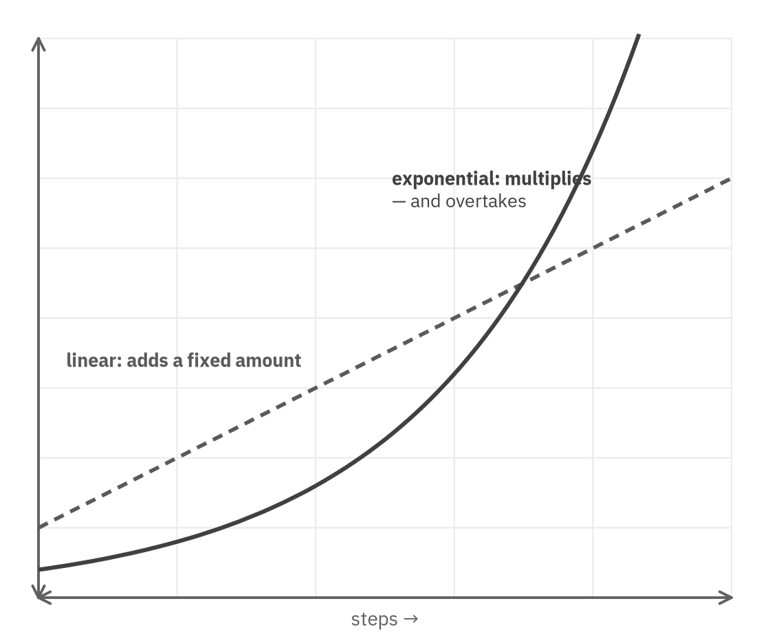
Figure 1. Linear change adds a fixed amount each step; exponential change multiplies. The exponential starts lower yet overtakes.

Worked example: adding versus multiplying. Start both at 3. A linear model that adds 3 each step gives $3, 6, 9, 12, \dots$ An exponential model that multiplies by 2 each step gives $3, 6, 12, 24, \dots$ The two agree at first and then part ways fast: the line climbs by a steady 3, while the curve doubles, and doubling soon dwarfs adding.

This gives a test you can run on a table of values at equally spaced inputs. If the differences between consecutive outputs are constant, the pattern is linear. If the ratios between consecutive outputs are constant, the pattern is exponential, and that common ratio is the base. For the outputs $12, 18, 27, 40.5$ the ratios are $\frac{18}{12} = \frac{27}{18} = \frac{40.5}{27} = 1.5$, so the base is $1.5$.

Distinguish exponential growth from exponential decay

The base decides the direction. When $b > 1$, each step multiplies by more than one, so the quantity grows. When $0 < b < 1$, each step multiplies by a fraction, so the quantity decays toward zero. Same form, opposite behavior, and the graph tells them apart at a glance.

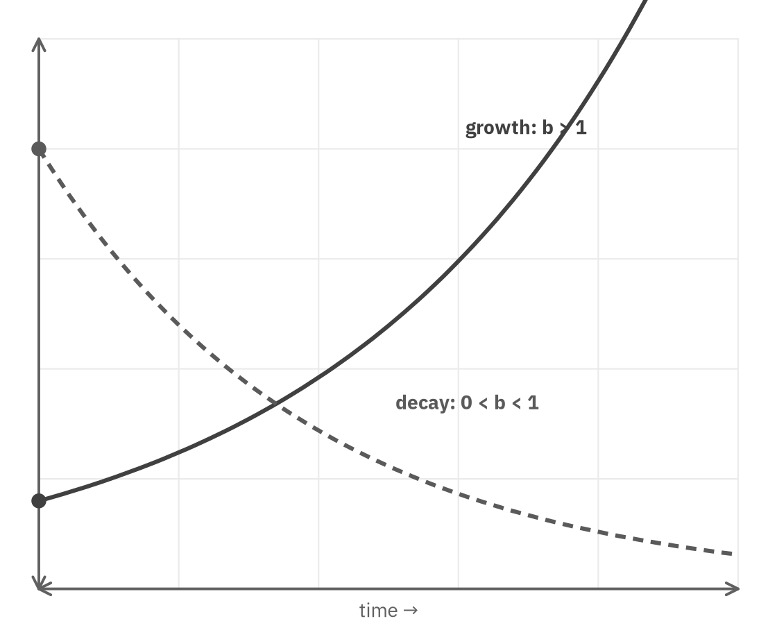
Figure 2. A base above one rises; a base between zero and one falls. The starting value is the $y$-intercept, the output at $x = 0$.

In a real model the base is usually written through a rate. Growth at rate $r$ per period multiplies by $(1 + r)$ each period, giving $y = a(1+r)^t$; decay at rate $r$ multiplies by $(1 - r)$, giving $y = a(1-r)^t$. The rate is a decimal, so eight percent is $r = 0.08$, and the factor is $1.08$ for growth or $0.92$ for decay.

Decay by repeated halving is common enough, and shows up in different-sounding language often enough, that it is worth naming on its own: a half-life is simply the base $\frac{1}{2}$, and the exponent counts how many half-lives have passed.

Worked example: fraction remaining after several half-lives. A substance has a half-life of 6 years. What fraction of the original amount remains after 18 years? Count the half-lives: $18 \div 6 = 3$ half-lives have passed. Each one multiplies the remaining amount by $\frac{1}{2}$, so $\left(\frac{1}{2}\right)^3 = \frac{1}{8}$. The common error is subtracting instead of multiplying, treating three half-lives as losing three equal chunks rather than three repeated halvings. Halving compounds, exactly like any other repeated percent change.

Convert percent increase or decrease to an exponential factor

The bridge from everyday language to an exponential model is one idea: a percent change is a multiplying factor. Increasing a quantity by $p$ percent multiplies it by $\left(1 + \frac{p}{100}\right)$; decreasing it by $p$ percent multiplies by $\left(1 - \frac{p}{100}\right)$. A single change is one multiplication; a repeated change is that factor raised to a power.

Worked example: one change, then many. A price of 80 increased by 25 percent multiplies by $1.25$: $80(1.25) = 100$. A population of 100 that grows 10 percent per year for 3 years multiplies by $1.1$ three times: $100(1.1)^3 = 100(1.331) = 133.1$. The exponent counts the repetitions; the base is the one-step factor.

Create and interpret exponential functions in context

Putting it together, you can build a model from a description and read one back into words. To build, identify the starting amount (that is $a$), the one-step factor (from the growth or decay rate, that is $b$), and what the exponent counts. To read, reverse it: the coefficient is the initial value, the base is the per-period factor, and subtracting one from the base recovers the rate.

Worked example: build a model, then read one. "A colony of 200 bacteria triples every hour." The starting amount is 200 and the factor is 3 per hour, so $N = 200(3)^t$. Reading back, in $y = 1500(1.04)^t$ the initial value is 1500, the factor is $1.04$, and since $1.04 = 1 + 0.04$, the growth rate is 4 percent per period.

When interest is compounded more often than once per period, the rate is split across the smaller periods and the exponent counts them: $A = P\left(1 + \frac{r}{n}\right)^{nt}$ applies a rate $r$ compounded $n$ times per year over $t$ years. The structure is the same exponential model, with the per-step factor and the step count adjusted to match how often the compounding happens.

Solve an exponential model for an earlier value or time

Two variations run the model-reading skill in directions this chapter has not yet asked for. The first hides the base inside a relationship between consecutive outputs rather than stating it directly.

Worked example: find the base from a recursive relation. For $f(x) = ab^x$, $f(n) = 1.25 \cdot f(n-1)$ for every integer $n$. What is $b$? The ratio between any output and the one before it is exactly the base, by definition of an exponential model: $\dfrac{f(n)}{f(n-1)} = b$. So $b = 1.25$ directly. The relation was already stating the base in a different form; no equation needed to be built or solved.

The same idea finds the base from two outputs that are several steps apart. If $f(1) = 6$ and $f(4) = 162$, divide to cancel $a$: $\dfrac{f(4)}{f(1)} = b^3 = \dfrac{162}{6} = 27$, so $b = 3$.

The second variation runs the model backward: given a target output, solve for the exponent, the amount of time or the number of periods, rather than reading a value forward.

Worked example: solve for the exponent. A quantity follows $N = 300(2)^t$. For what $t$ is $N = 2400$? Isolate the exponential factor first, then match it to a recognizable power: $2400 = 300(2)^t$ gives $8 = 2^t$. Since $8 = 2^3$, the exponents must agree: $t = 3$. Recognizing the target as a power of the given base is what turns this into arithmetic; when the numbers do not divide so cleanly, Desmos can solve the same equation by graphing $y = 300(2)^x$ and $y = 2400$ and reading the intersection.

Compare linear and exponential models

One comparison is worth carrying out of this section, because the test returns to it: given enough room, growing exponentially (base greater than one, positive coefficient) overtakes any linear growth, no matter how steep the line or how gentle the curve begins. A line that adds a hundred each step will, for a while, stay far ahead of a quantity that merely doubles from one. For $y = ab^x$ with $a > 0$ and $b > 1$, exponential growth eventually exceeds any linear function as $x$ increases without bound. When a question contrasts a fixed amount added against a fixed positive factor greater than 1 multiplied, the multiplied one eventually wins in the long run.

Chapter summary

Exponential change multiplies rather than adds. The exponent rules move powers around, fractional exponents are roots, and an exponential model $y = ab^x$ reads as a starting value $a$ times a per-step factor $b$: growth when $b > 1$, decay when below one. A percent change is just that factor, $(1 + r)$ or $(1 - r)$, and a repeated change raises it to a power. Build the model by naming the start and the factor; read one by reversing the steps. And remember the long-run truth the test keeps returning to: growth with a base above one eventually overtakes any linear rate, given enough room.