Inference, margin of error, and statistical claims
A study measures a few and reasons to the many. What it may honestly claim, about cause and about whom, is decided not by the data but by how the data was gathered.
This chapter asks not what the numbers are but what they are allowed to say. A study never measures everyone; it measures a sample and reasons outward to a whole population. Whether that reasoning is sound (whether a result generalizes beyond the people studied, and whether it shows that one thing causes another) depends almost entirely on how the study was designed. This is where the caution from the scatterplot chapter gets its full answer: association becomes evidence of cause only under a specific condition, and a result describes a population only under another. Knowing those two conditions, and reading a study against them, is what this chapter trains.
Representative samples and population inferences
A sample is the group actually measured; the population is the larger group you want to know about. A number computed from the sample (a sample mean, a sample percentage) is an estimate of the corresponding true value in the population. The estimate is trustworthy as a stand-in for the population when the sample is chosen at random from the population you want to describe. Random selection is the design feature that justifies generalizing, because it keeps the sample from systematically over- or under-representing any part of the population in expectation. Without random selection, the sample may describe only itself.
Note the boundary of the claim: a random sample of a city's residents lets you generalize to that city's residents, and no farther. Other cities, other years, and other kinds of people were never sampled.
Margin of error around a sample estimate
A sample estimate need not equal the population value, so a study may report the estimate together with a margin of error to describe its uncertainty. A poll finding 52 percent support with a margin of error of 3 points is really saying the true population figure plausibly lies between 49 and 55 percent. The recipe is always the same: estimate minus margin to estimate plus margin. All else equal, increasing the sample size generally decreases the margin of error and makes the estimate more precise.
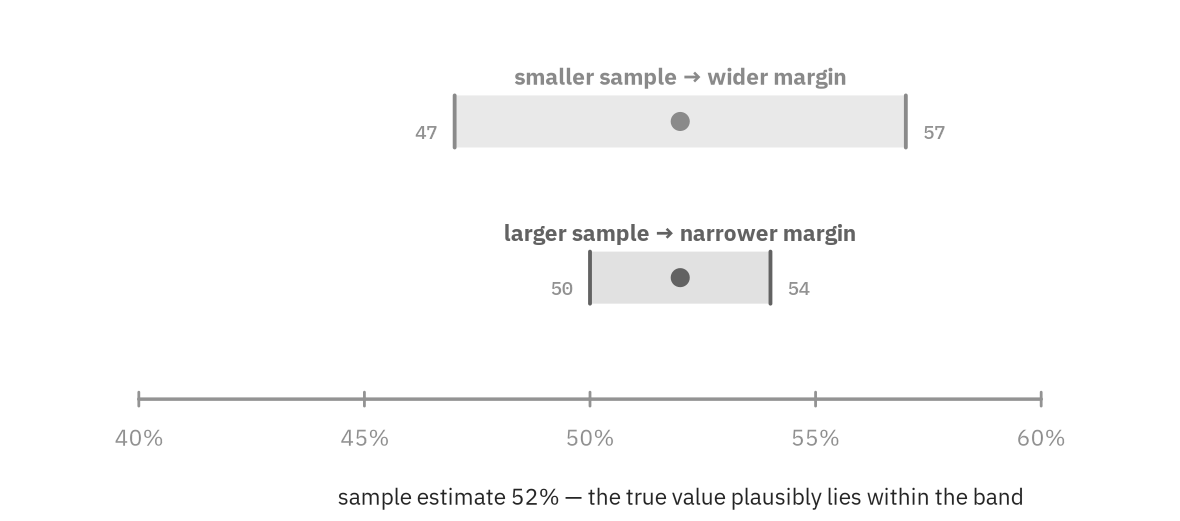
Figure 1. A sample estimate is a band, not a point. A larger sample narrows the band, pinning the true value down more tightly.
A confidence interval is this same band given a confidence level: a 95 percent confidence interval of, say, 48 to 56 means the procedure produces intervals that capture the true value most of the time, so those bounds are the plausible range for it. A value inside the interval is consistent with the data; a value outside is not well supported. The midpoint of the interval is the sample estimate, and half its width is the margin of error. In the example, the estimate is 52 and the margin of error is 4.
Two habits protect you from the usual traps. First, never read the interval as the spread of the individual data values; it describes the plausible values of the population figure. Second, when a claim sits inside the interval (for example, "support is 50 percent" when the interval is 49 to 55), the data are consistent with it, so the study cannot rule it out. This matters for "who is winning" questions: if the interval for a candidate's support includes values on both sides of 50 percent, the poll does not establish a lead.
Random sampling versus random assignment
Two separate uses of randomness sit at the heart of study design. They answer different questions and license different conclusions, and keeping them distinct is the single most valuable idea in this chapter.
Random sampling vs. random assignment
Random sampling: randomly choosing who is in the study from the population. This is what lets results generalize to that population.
Random assignment: randomly choosing who receives which treatment among the participants. This is what lets a difference be attributed to cause.
They are independent choices: a study can use either, both, or neither, and each conclusion it earns comes from a different one.
Observational studies versus experiments
The distinction in randomness produces the distinction in study type. In an observational study, the researcher only watches, recording who already does what, and so can detect that two things go together but can never rule out that some third factor drives both. In an experiment, the researcher intervenes, using random assignment to impose the treatment, which tends to balance potential confounders across the groups and so supports a causal conclusion. The grid below collapses everything into one picture: the columns ask whether the sample was random, the rows whether the assignment was, and each cell names exactly what may be concluded.
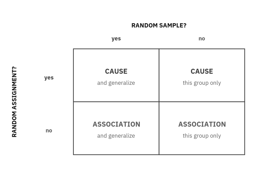
Figure 2. What a study earns: random assignment buys cause; random sampling buys generalization. Each is needed for its own conclusion.
Read the grid as two independent switches. Random assignment moves you from "association" up to "cause." Random sampling moves you from "this group only" out to "generalizes to the population." A study earns a conclusion only on the axis whose randomness it actually used.
Match generalization and causation claims to study design
A common task is matching the study design to the conclusions it can support.
- An experiment with random assignment but volunteer participants can claim cause, but only for people like those volunteers, since no random sample was drawn.
- A random survey with no assigned treatment can generalize its finding to the whole population but can show only association, never cause.
- The strongest claim, both cause and generalization, requires both randomizations.
- The weakest, an observational study on a self-selected group, supports only an association among those particular people.
In every case, you match the study's two design choices to the two axes and read off precisely what is earned, no more.
Worked example: read a study against the grid. A study randomly assigns volunteer patients to a drug or a placebo; the drug group improves more. The patients were not randomly sampled.
Random assignment was used, so a causal claim is justified: the drug likely caused the improvement.
Random sampling was not, so the result holds only for patients like these volunteers; it may not generalize to the broader population.
Conclusion: cause, but not generalization. That is the upper-right cell of the grid.
Sampling bias and limits on generalization
Finally, the most common way a study goes wrong: a sample that is not random and so does not represent its population, a source of bias.
- A voluntary-response sample, made of only those who chose to reply, over-represents people with strong opinions.
- A convenience sample, made of whoever was easiest to reach, over-represents the nearby and the available.
In both, the sample tilts away from the population in some systematic direction, so the estimate it gives is off in that direction no matter how large the sample grows. Increasing the size of a systematically biased sample does not remove the bias; it can produce a more precise estimate of the wrong target. Random selection is what reduces this systematic tilt, which is why every claim to generalize rests on it. It reduces sampling error in expectation, though it does not eliminate every source of nonresponse or measurement error.
Strategy checklist
- Ask two questions of every study: Was the sample random? (generalization) and Was the assignment random? (cause).
- Build an interval as estimate margin of error; a claim inside it is consistent with the data, a claim outside it is not.
- A larger sample narrows the margin of error but never repairs a biased sampling method.
- Limit every conclusion to the population actually sampled, and to association unless treatments were randomly assigned.
With that, the four domains of the test's mathematics are complete; what remains is putting them to work.