Probability and Conditional Probability

Probability and conditional probability

Probability is a proportion of outcomes, and the hard part is almost never the arithmetic. It is reading the word "given," which quietly shrinks the group you are dividing by.

Probability measures how likely an outcome is, on a scale from 0 (impossible) to 1 (certain), and at heart it is the proportional reasoning of this domain's first chapters pointed at chance. For equally likely outcomes it is a simple ratio, favorable outcomes over total outcomes. On this test it most often appears as data in a two-way table. The arithmetic stays easy throughout; the difficulty is entirely in reading which outcomes count and, above all, which group you are dividing by. That second question is what the word "given" controls, and it is where this chapter concentrates its attention.

Favorable outcomes over a sample space

For a process whose outcomes are equally likely, the probability of an event is the number of outcomes in the event divided by the total number of outcomes:

$P(\text{event}) = \frac{\text{number of favorable outcomes}}{\text{number of possible outcomes}}$

Because it is a proportion, it always lands between 0 and 1. The probability that an event does not happen, its complement, is simply $1$ minus the probability that it does. The complement is a quiet workhorse: when an event is awkward to count directly, counting the opposite and subtracting from 1 is often far easier.

Estimate probability from observed frequencies

When the outcomes are not equally likely, or when you simply have a record of what happened, probability is estimated by relative frequency: the fraction of observed cases in which the event occurred. If 90 of 150 surveyed households own a pet, the probability that a randomly chosen household owns a pet is taken to be $\frac{90}{150} = 0.6$. This form turns any table of counts into a source of probabilities. The same idea also runs in reverse: to predict how many cases to expect in a larger group, multiply the probability by the group size.

Read joint, marginal, and conditional frequencies from two-way tables

A two-way table sorts a group by two characteristics at once, with row and column totals around the edges. One table can support joint, marginal, and conditional probabilities. Read it carefully: the inner cells are joint counts (both characteristics at once), the margins are single-characteristic totals, and the grand total sits in the corner.

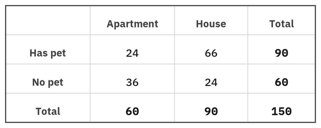
Figure 1. A two-way table of 150 households by housing and pet ownership. Inner cells are joint counts; the margins are totals.

Worked example: read probabilities from the table. Using the 150 households above, with the grand total as the denominator:

A single characteristic: $P(\text{has pet}) = \frac{90}{150} = 0.6$, and by the complement $P(\text{no pet}) = 1 - 0.6 = 0.4$.

Both at once (joint): $P(\text{apartment and has pet}) = \frac{24}{150} = 0.16$, straight from the inner cell.

A margin: $P(\text{apartment}) = \frac{60}{150} = 0.4$, using the column total.

Each of these divides by the grand total 150, because the chosen household could be anyone in the table.

Conditional probability: the conditioned group is the sample space

Now the central idea. A conditional probability asks for the chance of one event given that another is already known to be true, and that knowledge changes the question by shrinking the group you are choosing from. "Given that the household lives in an apartment" means you are no longer choosing from all 150; you are choosing only from the 60 apartment households. The condition becomes the new denominator.

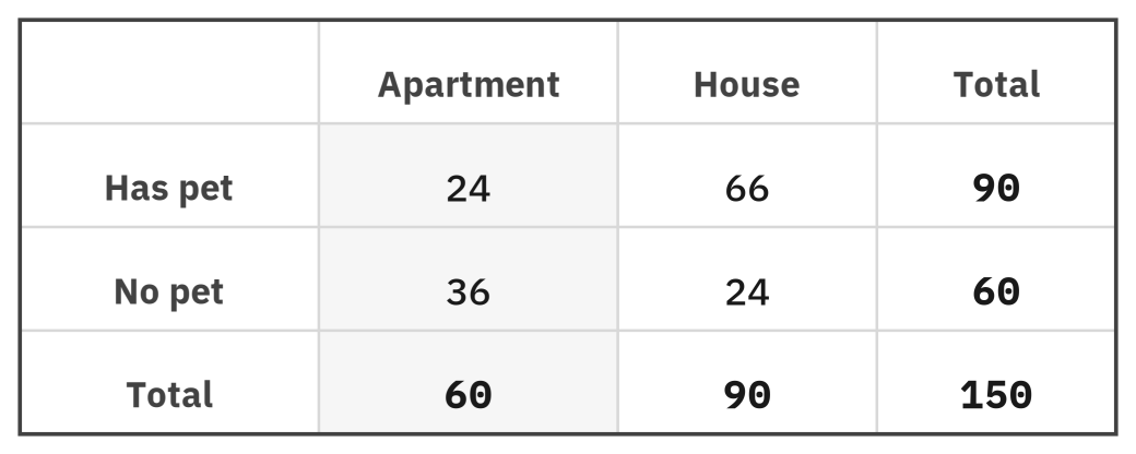
Figure 2. "Given the household is in an apartment" restricts attention to the apartment column: the denominator becomes 60, not 150.

Worked example: compute a conditional probability. $P(\text{has pet} \mid \text{apartment})$: restrict to the apartment column (total 60), then count pet owners within it (24):

$P(\text{has pet} \mid \text{apartment}) = \frac{24}{60} = 0.4$.

Reverse the condition and the denominator changes entirely. $P(\text{apartment} \mid \text{has pet})$ restricts to the pet-owner row (total 90):

$P(\text{apartment} \mid \text{has pet}) = \frac{24}{90} \approx 0.267$.

Same joint cell of 24, two different answers, because the condition picks the denominator, and the two conditions name different groups.

That last point is the one the test rewards most: $P(A \mid B)$ and $P(B \mid A)$ are not the same, because they divide the same overlap by different totals. Whenever you see "given," find the group it names, make that total your denominator, and count the favorable cases inside it. The phrases "of the," "among," and "for those who" often signal a condition in disguise: "Of the satisfied commuters, what fraction use transit?" is a conditional probability whose denominator is the satisfied total.

Intersection, union, and complement rules

For the probability of $A$ or $B$, adding $P(A)$ and $P(B)$ double-counts the overlap, so you subtract it back:

$P(A \text{ or } B) = P(A) + P(B) - P(A \text{ and } B)$

For independent events, where one outcome does not affect the other, the probability of both is the product $P(A) \times P(B)$. Paired with the complement, this handles "at least one" questions cleanly. You can test independence with a table: events $A$ and $B$ are independent only if $P(A \mid B) = P(A)$. If conditioning on $B$ changes the probability of $A$, the events are not independent.

Worked example: use the or-rule and the complement. $P(\text{apartment or has pet})$, from the household table:

$\frac{60}{150} + \frac{90}{150} - \frac{24}{150} = \frac{126}{150} = 0.84$.

Subtracting the overlap 24 prevents counting the apartment pet owners twice.

For "at least one," use the complement: if each of three independent trials succeeds with probability 0.2, then

$P(\text{at least one}) = 1 - (0.8)^3 = 1 - 0.512 = 0.488$.

Counting the one way nothing happens is far easier than counting all the ways something does.

Geometric probability from area ratios

Not every probability question counts discrete outcomes from a table. When an outcome is chosen uniformly from a continuous region, a point landing anywhere in a square with equal likelihood, say, probability is read as a ratio of areas instead of a ratio of counts: the area of the favorable region over the area of the whole sample space.

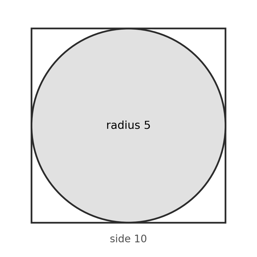
Figure 3. A point chosen uniformly in the square is equally likely to land anywhere in it; the circle marks the favorable region.

Worked example: a circle in a square. A point is chosen uniformly at random from a square of side 10. A circle of radius 5 lies entirely inside the square, as shown. What is the probability the point lands inside the circle?

Probability is the favorable area over the total area:

$P = \frac{\text{area of circle}}{\text{area of square}} = \frac{25\pi}{100} = \frac{\pi}{4}$

The count-based formula still applies; area simply plays the role that a count of discrete outcomes played in a two-way table. Using the circumference or the radius alone in place of area is the usual error.

The same area logic extends to two overlapping events at once, drawn as regions inside a rectangle representing the whole sample space. Reading it is the same denominator discipline as a two-way table, only drawn geometrically instead of counted in cells.

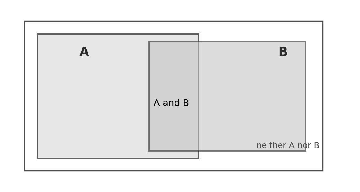
Figure 4. An area model: the whole rectangle is the sample space; overlapping regions represent events $A$ and $B$ happening together.

Worked example: read a conditional probability from an area model. The rectangle above has a total area of 120. Region $A$ covers 50, region $B$ covers 60, and their overlap covers 20. What is $P(A \text{ and } B)$? What is $P(A \mid B)$?

$P(A \text{ and } B)$ is the overlap over the whole space: $\frac{20}{120} = \frac{1}{6}$.

$P(A \mid B)$ restricts attention to region $B$ alone, exactly as "given" restricted a two-way table to one column: $\frac{20}{60} = \frac{1}{3}$.

The whole area, 120, is the denominator only for an unconditional probability; the moment a condition is named, the denominator shrinks to that condition's own region.

Strategy checklist

1. Decide whether the question is unconditional (grand total as denominator), joint (one inner cell over the grand total), or conditional (the "given" group's total as denominator).
2. Underline the "given" group before you touch the numbers.
3. For "or," subtract the overlap. For "at least one," use the complement.
4. For independent events, multiply. To test independence, compare $P(A \mid B)$ with $P(A)$.
5. For "how many would you expect," multiply the probability by the new group size.
6. For uniform points in a region, use the ratio of areas.