One-Variable Data: Distributions, Center, and Spread

One-variable data: distributions, center, and spread

A single list of numbers can be summarized by where it centers and how far it spreads. The reasoning the test rewards is knowing how those summaries shift when the data does.

When data comes as a single list of values (test scores, heights, incomes), two questions organize almost everything you can ask about it: where does it center, and how spread out is it? The first is answered by the mean, the median, or the mode; the second by the range and the standard deviation. None of these is hard to compute. What the harder questions test is your grasp of how each summary behaves: how the mean shifts when a value is added, why the median shrugs off an outlier the mean cannot, and what happens to the spread when every value is scaled. That behavior, not the arithmetic, is the real content of this unit.

Compare mean, median, and mode

Three numbers compete to describe the center of a list. The mean is the ordinary average, the sum divided by the count. The median is the middle value once the list is ordered (the average of the two middle values when the count is even). The mode is the value that appears most often. On a roughly symmetric list these three sit close together; their differences become important precisely when the list is not symmetric.

The most useful mean questions run backward. Because the mean ties together the sum and the count, knowing any two of those three recovers the third, and that is the engine behind a whole family of harder problems.

Worked example: run the mean backward

The mean of five numbers is $14$. Four of them are $10$, $12$, $15$, and $18$. Find the fifth.

A mean of $14$ over five numbers means the total is $5 \times 14 = 70$. The four known values sum to $55$, so the fifth value is $70 - 55 = 15$.

The move is always the same: turn the mean into a sum, then work with the sum.

Compute means from frequency tables and weighted data

When data arrives in a frequency table, each value paired with how many times it occurs, you read the center without writing the list out. The mean weights each value by its frequency; the median is found by counting inward to the middle position, using a running total of the frequencies.

Worked example: median from a frequency table

Value	Frequency	Running total
$2$	$3$	$3$
$5$	$4$	$7$
$8$	$5$	$12$
$11$	$8$	$20$

The total count is $20$, so the median is the average of the $10$th and $11$th values in order. Through the value $2$ we reach position $3$; through $5$, position $7$; through $8$, position $12$. So positions $8$ through $12$ are all the value $8$, including both the $10$th and $11$th.

$\text{median} = \frac{8 + 8}{2} = 8$.

Counting positions through the running total is the whole skill; never list out twenty numbers.

A close relative is the weighted mean, which combines groups of different sizes. You cannot simply average the group averages unless the groups are the same size; instead, weight each average by its group's count.

Worked example: combine two group means

One class of $18$ students averaged $78$; a second class of $12$ averaged $88$. Find the combined average of all $30$.

Recover each group's total, add, and divide by the full count: $\frac{18 \times 78 + 12 \times 88}{30} = \frac{1404 + 1056}{30} = \frac{2460}{30} = 82$.

Averaging $78$ and $88$ to get $83$ would be wrong, because the larger class pulls the combined mean toward its own average.

Read distributions from histograms and dot plots

Two graphical displays organize a long list of values without listing every one, and both group values into bins or stack them by value. A histogram groups values into intervals; SAT-style displays commonly use equal-width bins, and the graph's labels show how frequency is represented for each interval. Because a histogram groups values, it tells you how many observations fall in a range, never the exact value of any one of them.

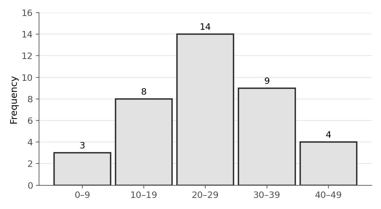
Figure 1. A histogram groups values into equal-width intervals; bar height is the frequency in that interval.

Worked example: read a histogram correctly

The tallest bar above spans $20$ to $29$, with a frequency of $14$. What must be true?

More observations fall in the interval $20$ to $29$ than in any other interval shown. Nothing more specific can be said: the histogram does not reveal the exact values inside that bar, or their mean, only the count within the range.

A common misread is to treat the tallest bar as revealing a single most-common value; a histogram groups values, so individual repeats inside a bin stay invisible.

A dot plot keeps every individual value visible instead of grouping them, stacking one dot per observation above its value on a number line. It is most useful for smaller data sets, where a histogram's bins would hide more than they reveal.

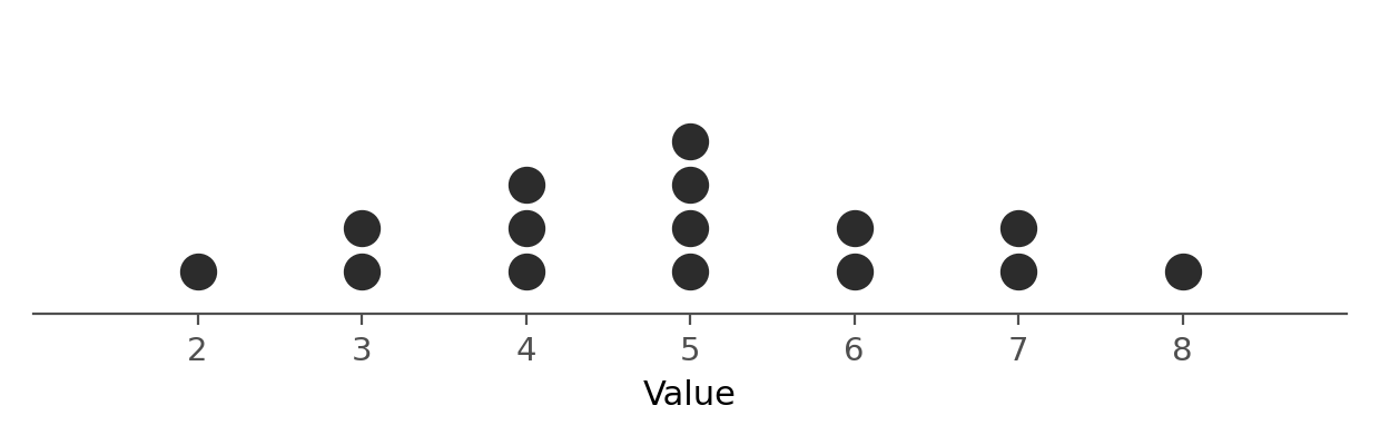
Figure 2. A dot plot stacks one dot per observation above its value, keeping every individual value visible.

Worked example: recover the median from a dot plot

The dot plot above shows $15$ values. What is the median?

With $15$ values, the median is the $8$th value once they are ordered. Reading left to right and counting dots: $2, 3, 3, 4, 4, 4, 5$. The $8$th dot lands on $5$.

Unlike a histogram, a dot plot lets you count individual observations directly, which is exactly what finding a median from raw data requires.

Compare spread using range and standard deviation

Center is only half the picture; two lists can share a mean yet look nothing alike. Spread measures how far the values stray from the center. The simplest measure is the range, the largest value minus the smallest: quick, but driven entirely by the two extremes. The far more informative measure is the standard deviation, which captures the typical distance of a value from the mean. You will not compute it by hand on this test, but you must reason about it: a list whose values huddle near the mean has a small standard deviation, while one whose values are flung wide has a large one.

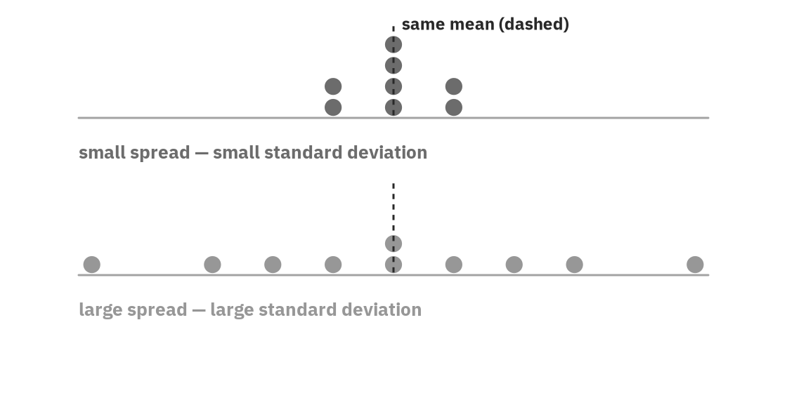
Figure 3. Two lists can share a mean and differ entirely in spread. Standard deviation measures the typical distance from that shared center.

So when a question shows two distributions with the same center and asks which has the greater standard deviation, you are being asked to see the spread, not calculate it: the more the values scatter away from the middle, the larger the standard deviation.

Worked example: different means, the same standard deviation

Data set $A$ has a mean of $50$ and a standard deviation of $8$. Data set $B$ is formed by adding $10$ to every value in set $A$. What are the mean and standard deviation of set $B$?

Adding the same constant to every value slides the whole distribution without changing how spread out it is: the mean shifts by that constant, $50 + 10 = 60$, but the standard deviation is unchanged at $8$. Two distributions can therefore look nothing alike in center while sharing an identical spread; the question tests whether you separate the shift, which moves the mean, from the shape, which fixes the standard deviation.

Read quartiles and interquartile range from box plots

A scope note: box plots themselves are a named current testing point, so locating the minimum, quartiles, median, and maximum on one is worth knowing. Computing the IQR as its own named quantity is not itself a current testing point; treat it as a natural byproduct of reading the box, not a separate fact to drill.

A box plot summarizes a full distribution using five landmark values: the minimum, the first quartile ($Q_1$), the median, the third quartile ($Q_3$), and the maximum. Quartiles split the ordered data into four equal groups; $Q_1$ is the median of the lower half, $Q_3$ is the median of the upper half. The box itself spans $Q_1$ to $Q_3$, the middle half of the data, with whiskers reaching out to the minimum and maximum.

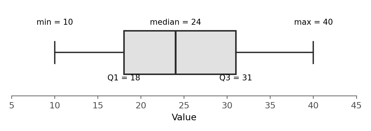
Figure 4. A box plot: the box spans $Q_1$ to $Q_3$ with the median marked inside; whiskers reach the minimum and maximum.

The interquartile range, IQR, is the width of the box, $Q_3 - Q_1$, and it measures spread the same way the range does, but resistant to outliers, since it ignores the most extreme quarter on each end.

Worked example: find the IQR from a box plot

The box plot above has $Q_1 = 18$ and $Q_3 = 31$. What is the IQR?

$\text{IQR} = Q_3 - Q_1 = 31 - 18 = 13$.

Confusing the IQR with the whisker-to-whisker span, the full range, is the usual slip; the IQR is the width of the box alone, the middle $50$ percent of the data.

Describe distribution shape, center, spread, and outliers

How a list is shaped (symmetric, or stretched out to one side) decides how its center measures relate. In a symmetric distribution the mean and median nearly coincide. But when a long tail stretches to one side, the values out in that tail drag the mean toward them, while the median, which only cares about position, barely moves. The result is a reliable signal.

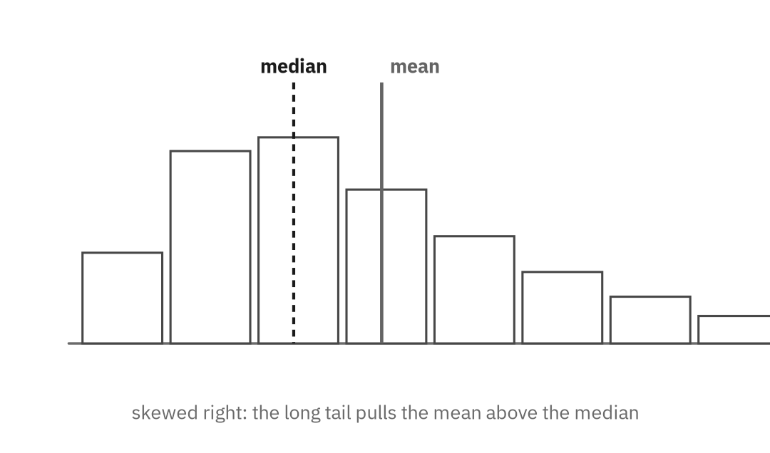
Figure 5. In a right-skewed distribution the long tail pulls the mean above the median; the median stays near the bulk of the data.

How skew changes the mean and median

• Symmetric: mean and median are nearly equal.
• Skewed right (long tail of high values): mean $>$ median.
• Skewed left (long tail of low values): mean $<$ median.

This runs in both directions. Shown a shape, you can predict the order of mean and median; told that the mean exceeds the median, that pattern typically points to a right skew, a useful heuristic rather than a guarantee for every possible dataset.

Choose median and IQR when outliers distort mean and range

An outlier, a single value far from the rest, exposes the deepest difference between the mean and the median. The mean, built from the sum, feels every value in full, so one extreme number can drag it a long way. The median, built from position, registers an outlier as just one more value at the end and scarcely moves. The median is resistant; the mean is sensitive.

Worked example: watch an outlier move each measure

A list of nine values has mean $50$ and median $50$. The largest value, $80$, is replaced by $200$, a jump of $120$.

The median depends only on the middle position, which is unchanged, so it stays at $50$.

The mean rises by the added amount spread over nine values: $\frac{120}{9}$, about $13.3$, lifting it to roughly $63.3$.

One value moved; the mean followed it and the median did not. That gap is the whole idea of resistance.

Predict how shifts and scaling affect summary statistics

A final behavior worth knowing cold: what happens to these summaries when every value in a list is changed the same way. Two cases cover the test. Adding a constant to every value slides the whole list along: the mean and median both shift by that constant, but the spread does not change, because every value moved together. Multiplying every value by a constant scales everything: the mean, the median, and the standard deviation all multiply by that same factor.

How transformations change center and spread

• Add $c$ to every value: mean and median rise by $c$; range and standard deviation are unchanged.
• Multiply every value by $k$: mean and median multiply by $k$; range and standard deviation multiply by $|k|$, since a spread cannot be negative.

Worked example: transform a whole list

A list has mean $20$ and standard deviation $4$. Every value is multiplied by $3$, and then $5$ is added.

Multiplying by $3$ scales both: the mean becomes $60$ and the standard deviation becomes $12$. Adding $5$ shifts the mean to $65$ but leaves the standard deviation at $12$, since a shift moves every value together.

New mean $= 3(20) + 5 = 65$, new standard deviation $= 3 \times 4 = 12$. The order matters for the mean but not for the spread, which only the multiplication touched.

Choose center or spread measures that match the question

All of this serves one judgment: which summary honestly represents the data. For a roughly symmetric list, the mean is the natural center. For a strongly skewed one, household incomes pulled upward by a few very high earners is the standard example, the median better captures a typical value, because the mean is inflated by the tail. The test often frames this as a choice: which measure best describes the center, and would the mean sit above or below the median? Read the shape, name the skew, and the answer follows.

A checklist for one-variable data questions

1. If the mean is given, convert it to a sum right away: $\text{sum} = \text{mean} \times \text{count}$.
2. With groups of different sizes, weight each mean by its count.
3. With a frequency table, find the middle position and use running totals.
4. For a shift or scaling, track the mean and median through every step, and remember the spread ignores shifts and multiplies by $|k|$.
5. When a long tail or an outlier is present, expect the mean to move toward it and the median to stay put.

Summary. A list of numbers is summarized by its center and its spread, and the points live in how those summaries move. The mean ties sum to count, so most hard questions run it backward or weight it across groups. The median holds the middle position, which makes it resistant to outliers the sensitive mean chases. Shape links them: a tail to the high side pulls the mean above the median. Adding a constant shifts center but not spread; multiplying scales both. Read what the data is doing, decide which summary tells the truth about it, and the arithmetic is the easy part.