Two-variable data: models and scatterplots
When two quantities are measured together, a scatterplot shows their relationship and a fitted model summarizes it. The work that scores is interpreting that model, and knowing how far to trust it.
When each subject in a study is measured on two quantities at once (hours studied and a score, age and height, time and temperature), the data becomes a set of paired values, and a scatterplot is the picture of it: one dot for each pair. The scatterplot reveals whether the two quantities move together. If they do, a model, usually a line, can be drawn to summarize the relationship. From there the questions are almost entirely about interpretation: what the model's slope and intercept mean in the situation, how to use the model to predict, and, just as important, how far past the data you may responsibly reach.
Describe direction, strength, and form
Reading a scatterplot starts with three impressions, taken together.
- Direction. As one variable rises, does the other tend to rise (a positive association) or fall (a negative association)?
- Form. Do the points cluster around a straight line, or do they curve?
- Strength. Do the points hug the trend tightly, or scatter loosely around it?
These three words (direction, form, strength) are the vocabulary for describing any scatterplot before a single number is computed. A tight cloud sloping down to the right is a strong negative linear association. A loose cloud with no visible tilt is a weak or absent association.
Interpret and use a line of best fit
When the form is roughly linear, a line of best fit (also called a trend line) is drawn to summarize the relationship. Its defining feature is easy to overlook: it does not pass through every point, and usually passes through few or none. It summarizes the overall linear trend without needing to touch any observed point at all. The points still scatter; the line captures only the pattern running through them. On the SAT, the useful skill is interpreting a given fitted line and its predictions, not constructing one by eye.
Interpret slope and intercept in context
A line of best fit is still , and each piece carries a concrete meaning in the situation.
- The slope is a rate of change: the predicted change in for each one-unit increase in , in units of per unit of .
- The intercept is the predicted value of when .
Interpreting these correctly, in the units of the problem, is what the test asks again and again.
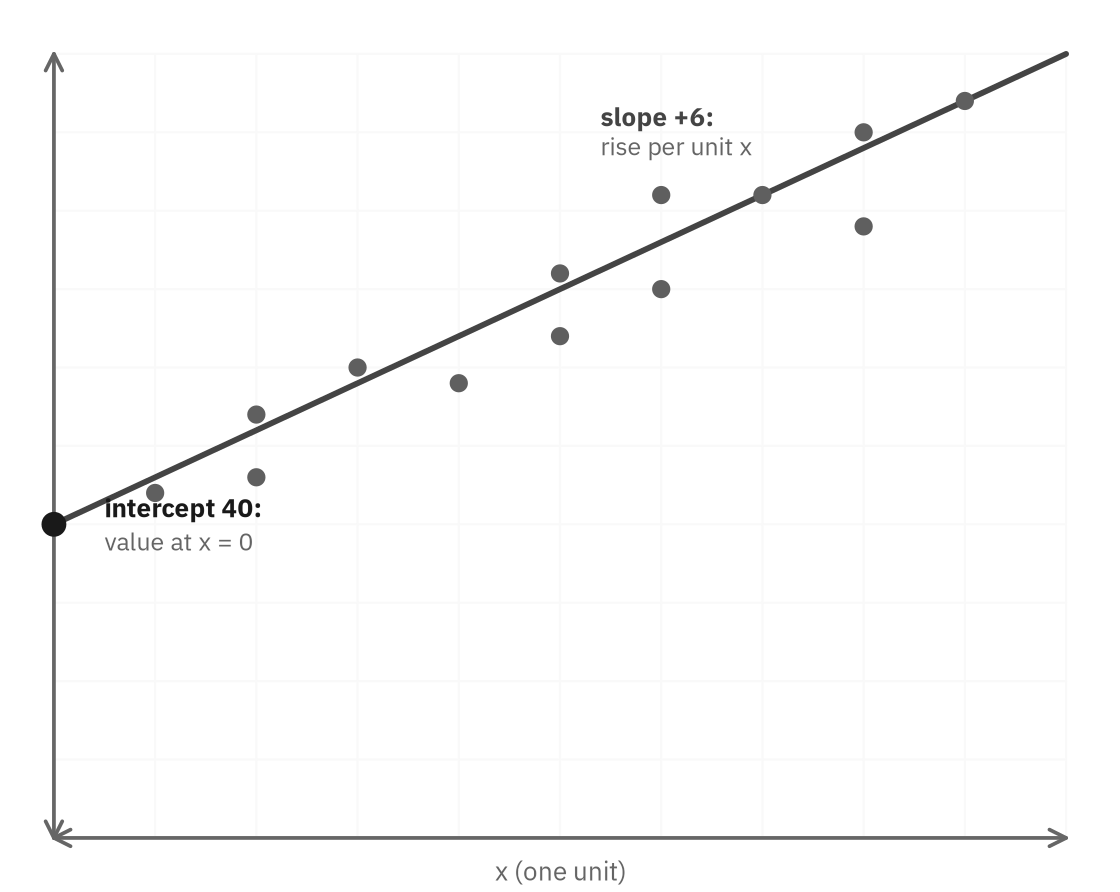
Figure 1. A line of best fit summarizes the trend. Its slope is the predicted change in per unit of ; its intercept is the predicted at .
Worked example: interpret a fitted model. A study models a channel's subscribers as , where is years since launch and is subscribers in thousands.
Slope 2.5: for each additional year, the model predicts about 2.5 thousand (that is, 2,500) more subscribers.
Intercept 18: at launch (), the model predicts 18 thousand subscribers.
Every interpretation question is this: attach the slope to "per unit of " and the intercept to "at ," both in the problem's own units.
Watch the units carefully. In the example, is in thousands, so a slope of 2.5 means 2,500 subscribers, not 2.5 subscribers. Wrong answer choices often swap the slope and intercept, or drop the units.
Use a model for prediction, and know the limits of extrapolation
A fitted model is a prediction machine: substitute an and read off the predicted . Predicting within the range of the data, called interpolation, is the model's home ground and is usually reliable. Predicting outside that range, called extrapolation, is where care is required, because there is no evidence the trend continues beyond where it was measured. A line fit to a battery draining over an hour might predict a charge below zero after two hours, which is meaningless. A population growing linearly for twenty years cannot be assumed to grow forever. The model is trustworthy across the data it summarizes, and progressively less so the farther past that range you push it.
Worked example: predict, then judge the prediction. Using , the prediction at years is thousand subscribers. That is an interpolation inside the data, and reasonable.
The prediction at years is thousand, but the data covered only the first several years, so this far extrapolation rests on the unproven hope that linear growth continues for decades.
The arithmetic is identical; the confidence is not.
Two other routine tasks use the same equation. To find when a model reaches a target, set equal to the target and solve for . To find a change in the prediction between two -values, multiply the slope by the change in ; the intercept cancels out. And if a line passes through two given points, find the slope from them, then move along the line from either point.
Interpret residuals as observed minus predicted
No model fits perfectly, and the gap between reality and the model has a name. The residual of a data point is its actual minus the value the model predicts there. A point above the line has a positive residual (the model under-predicted it); a point below has a negative one.
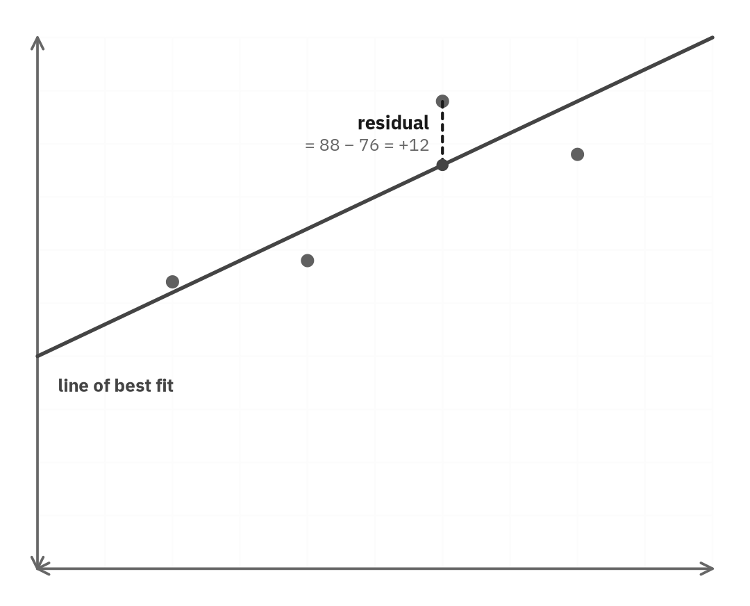
Figure 2. A residual is the vertical gap from a data point to the line: actual minus predicted. Points above the line have positive residuals.
The pattern of residuals also judges the model itself. If the residuals scatter randomly above and below zero, a line is a fair summary. But if they follow a pattern (negative at the ends and positive in the middle, say, or steadily growing), that pattern is evidence the true relationship is curved, and a line is the wrong shape for it.
A scope note: "residual" by itself is not a named Digital SAT testing point, while fitting quadratic and exponential models to a scatterplot is. Keep this idea for the model-fit intuition it builds, and give most of your practice time to choosing a model family.
Choose a model that matches the data pattern
Not every relationship is linear, and part of the skill is recognizing which shape the data calls for. If the quantity changes by a roughly constant amount for each step in , a line fits. If it changes by a roughly constant ratio, multiplying by about the same factor each step, an exponential curve fits. Reading the data's pattern of change, not just its upward or downward drift, tells you which model to reach for.
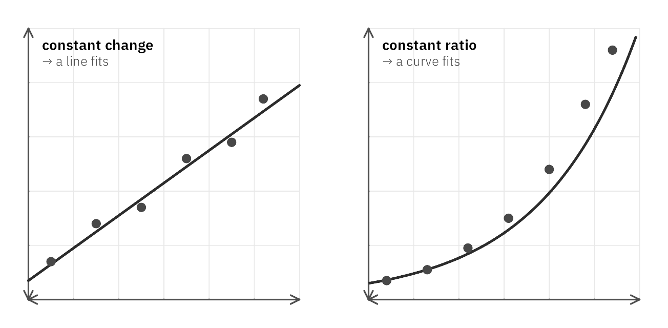
Figure 3. Constant change calls for a line; constant ratio (repeated multiplying) calls for an exponential curve.
A third pattern fits neither a line nor an exponential curve: a quadratic, where the amount of change itself changes by a constant amount each step. Reading the differences between consecutive values, and then the differences of those differences, tells the three apart.
| Check | If it is constant, the model is |
|---|---|
| Differences between consecutive -values | linear |
| Ratios of consecutive -values | exponential |
| Differences of the differences (second differences) | quadratic |
Worked example: recognize a quadratic pattern. A table shows -values 3, 7, 13, 21, 31 at equally spaced -values. Which model family fits best?
The differences between consecutive values are 4, 6, 8, 10, not constant, so it is not linear. Take the differences of those differences: 2, 2, 2, constant.
A constant second difference is the signature of a quadratic model; neither a line (constant first difference) nor an exponential curve (constant ratio) produces one.
Desmos handles the fitting itself once the family is chosen: enter the data as a table and fit y1 ~ ax12 + bx1 + c to get the coefficients directly, exactly as the linear and exponential regressions do.
Worked example: choose a model family directly from a scatterplot. The scatterplot below shows five data points. Which family, linear, quadratic, or exponential, best fits?
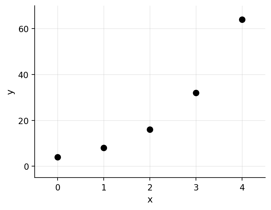
The points are not spread around a straight line, so linear is out. The curve does not simply bend once like a parabola's vertex; it accelerates continuously, climbing faster and faster as increases, each step roughly doubling the height of the last. That accelerating, ever-steepening shape, not just "curved," is the visual signature of exponential growth rather than a quadratic. Reading the shape directly from the picture, without building a table of differences, is the skill this scatterplot is testing.
Distinguish association from causal inference
One caution runs through the whole chapter. A strong association between two variables, even a tight, clean line, does not by itself establish that one causes the other. Two quantities can move together because one drives the other, because both are driven by some third factor, or by coincidence in a small sample. Whether a relationship is causal depends on how the data was collected, not on how strong the association looks, a distinction the next chapters take up in full. For now, hold the line: a scatterplot can show that two things move together, but moving together is not the same as one making the other happen.
Compare predictions from two competing models
When two models describe the same situation, a question can ask how the two compare: where they agree, and which pulls ahead afterward. Set the two expressions equal to find where the predictions match, then compare the rates to see which wins beyond that point.
Worked example. Model A predicts a store's weekly sales as ; model B predicts , where is the number of weeks since opening. For what value of do the two models agree, and which model predicts higher sales after that point?
Both models predict 750 at . Beyond that week, the comparison is a matter of rate, not another equation: model A grows by 50 each week against model B's 40, so model A overtakes model B and stays higher for every beyond 5. Checking confirms it: model A gives 900, model B gives 870.
Strategy checklist
- Describe the picture first: direction, form, strength.
- For a fitted line, name the slope as "change in per one unit of " and the intercept as " when ," with the problem's units.
- Predict by substituting; then ask whether the is inside the data range.
- Residual means actual minus predicted. Above the line is positive.
- To choose a family from a table, test differences, then ratios, then second differences.
- Never turn a tight association into a cause without a randomized experiment behind it.